ML-Multivariate Linear Regression
对于多变量的线性回归
通常多变量属于超平面,不能通过图像表示。一般的,我们令 $x_o^i=1,for(i\in1,…,m)$ 与 $\theta$ 的 $\theta_0$ 相对应。于是,对于一个X,它的维度为n+1,其中n为X的特征数量。
Gradient Descent for Multiple Variables
过去我们只讨论了n=1的情况,在这个情况下,我们分别迭代 \theta_0,\theta_1 ,即:
Repeat {
}
现在当变量很多时,显然像之前那样一一列举迭代 \theta 会很麻烦,于是我们使用向量的视角来看问题,即:
Repeat {
}
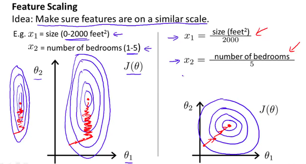
Feature Scaling
什么是Feature Scaling,为什么要使用它?
Feature Scaling: Make sure features are on a similar scale.
通过使得每个特征的取值范围变的一样,我们可以加速梯度下降。因为,$\theta$ 在小取值范围内能快速下降,在大取值范围内则下降的很慢。为了方便直观理解,使用Andrew课上的图,如下
Standardization: (Normal distribution 符合常态分布)
$x_i =\frac{x_i-\mu_i}{s_i}$
- $\mu_i$ 为均值
- $s_i$ 为标准差
Feature scaling:
$x_i=\frac{x_i- \underset{min}{x}}{\underset{max}{x}-\underset{min}{x}}$
Polynomial Regression
显然有时候线性的预测并不能满足我们的预期(与数据的拟合程度不高)。因为我们通过使Hypothesis function弯曲,使线性变为quadratic(二次), cubic(三次) 或者 square root(二次根号)。
E.g. If our hypothesis function is $h_\theta(x)=\theta_0+\theta_1x_1$
Then, we can create additional features based on $x_1$ like $h_\theta(x)=\theta_0+\theta_1x_1+\theta_2x_1^2$
本文由 Frank采用 署名 4.0 国际 (CC BY 4.0)许可
Machine Learning — 2021年4月20日
Made with ❤ and at Hangzhou.